Science - The Pigeon Roost

Season of Orion

With origins dating back to Homer’s epic Odyssey and one of the 48 constellations listed in Ptolemy’s Almagest, Orion provides a link for astronomy’s transformation between mythology and science. Many of the stars in Orion bear names rooted in Arabic, artifacts of the golden age of Islamic astronomy from 800 – 1450 A.D. Presently, NASA has designated Orion as the title for its deep space vehicle to carry humans to destinations beyond the Moon. As the winter solstice approaches, the most famous constellation begins to make its appearance high in the evening sky. Orion contains a rich tapestry of stars, nebulae, and history.

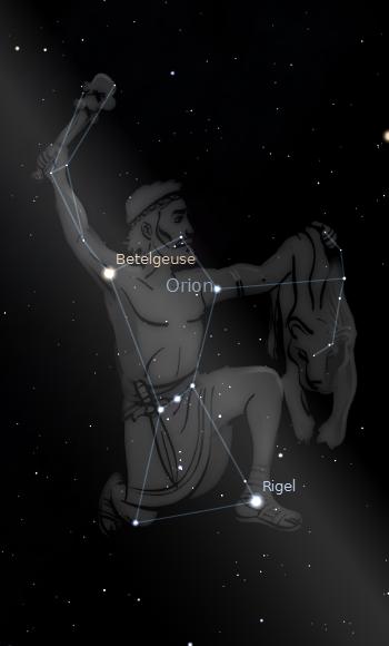
In early December, Orion rises above the eastern horizon around 7 PM. As the winter progresses, Orion rises earlier and earlier, meaning its zenith in the sky falls in the early evening hours making its visibility very prominent to anyone out and about at night. Located on the celestial equator, adjacent to the zodiacal constellations Gemini and Taurus, Orion is observable in both the Northern and Southern Hemispheres. The main seven stars are red or blue giants and are very luminous. To put the brightness of these stars in perspective, lets compare them to the Sun using a Hertzsprung-Russell (H-R) diagram.

Orion HR — Luminosity is in solar units (Sun = 1). Temperature is in Kelvins.

The Sun is represented by the yellow dot. You will note one of the quirks in the H-R diagram is that temperature, depicted by the horizontal axis, is scaled in reverse. That means hotter stars are on the left and cooler stars are on the right. All of the major seven stars of Orion are 10,000 to 100,000 times brighter than the Sun. In fact, most of the stars you see when looking at the night sky without the aid of a telescope will be brighter than the Sun. In the case of Orion, the stars are blue-white giants with the exception of Betelgeuse which is represented by the dot to the far right of the diagram. Betelgeuse is cooler than the Sun, how could it be so much brighter? The answer lies in its size.

Betelgeuse is so large the orbit of Mars could fit inside of it. A 100-watt light bulb is brighter than a 60-watt light bulb. However, ten 60-watt light bulbs are brighter than a single 100-watt light bulb. That is why Betelgeuse, despite being a relatively cool 3,500 K, is so luminous. Betelgeuse is a red giant, which means it is in the latter part of its life. A star becomes a red giant when all the hydrogen in its core has been burned up. As a star begins to fuse helium, the core becomes hotter, expanding the star much like hot air expands a balloon. Eventually, Betelgeuse will go supernova. Will we see this event? It’s possible, but not probable. A recent estimate predicts the supernova to occur in 100,000 years. To put that in perspective, the pyramids of Ancient Egypt were built about 5,000 years ago. But that’s not to say Betelgeuse is not interesting to observe now.

Looking at Orion, Betelgeuse occupies the upper left corner. Most stars appear to be white to the naked eye. With Betelgeuse, one can detect its red color. Most stars are too dim to activate the cones in our eyes that can discern color. Betelgeuse provides the opportunity to see the true color of a star without a telescope and/or camera. With a telescope, Betelgeuse provided astronomers the opportunity to make it the first star whose disk was resolved beyond a point of light. In 1996, the Hubble Space Telescope imaged the surface of Betelgeuse.

Betelgeuse, 1996. First image to resolve a stellar surface besides the Sun. Credit: Andrea Dupree (Harvard-Smithsonian CfA), Ronald Gilliland (STScI), NASA and ESA

Betelgeuse has attracted the curiosity of astronomers for centuries, and the roots of its distinct name is a legacy of that history. The word Betelgeuse is derived from the Arabic word Yad al-Jawza, which means forefront of the white-belted sheep. Many star names have their origins from the golden era of Islamic astronomy. One tip off of a word with Arabic origins is if it begins with “al”, which is equivalent to “the” in English. In Orion, the stars Alnitak (the girdle) and Alnilam (the belt of pearls) are two such examples. The Orion stars Mintaka (belt), Saiph (sword of the giant), and Rigel (rijl – foot) are also Arabic in nature. Of the seven major stars of Orion, Bellatrix is the outlier as it is derived from the Latin word for female warrior.

Scholars at the Abbasid Library in Baghdad, 1237. Many prominent astronomers from Central Asia traveled to Baghdad’s House of Wisdom to study. This library was sacked during the Mongol invasion of 1258. Credit: Wiki Commons.

The Arabic influence extends into math (algebra) and computer science (algorithm). As S. Frederick Starr describes in his book, Lost Enlightenment, the epicenter of this scientific golden age was in a region of Central Asia spanning from Eastern Iran to Western China and Kazakhstan to Northern Pakistan and India. As the Islamic Empire grew during this period, Arabic became the de facto language of science much as English is today. The Islamic astronomers were among the first to begin the process of challenging Ptolemy’s Earth centric model of the universe.

Ptolemy had listed Orion as a constellation in his Almagest. Note this title begins with the letters al. As you may have surmised, this is the Arabic translation of the title which is The Greatest Compilation and translates into Arabic as al-majisti. Ptolemy wrote Almagest in 150 A.D., and it survived as the primary star catalog until 1598 when Tycho Brahe published his thousand star catalog Stellarum octavi orbis inerrantium accurata restitutio. While Ptolemy was known to dabble in astrology, Almagest was concerned with the mathematical modeling of the motions of celestial objects. The mythology of Orion predates Ptolemy by several centuries.

While it can be difficult to discern mythological patterns in most constellations, it is easy to see how the Ancient Greeks viewed Orion as a hunter. In Greek mythology, Orion’s father was Poseidon. During the early 1970’s, a movie called The Poseidon Adventure, featuring an ocean liner capsized by a tidal wave, kickstarted a decade of disaster movies. The mythological Poseidon could walk on water and Orion inherited that trait. Orion, of course, was also a great hunter. So great, in fact, he threatened to kill every animal on Earth. This caused Orion to run afoul of Gaia, the goddess of Earth, who sent a scorpion to kill Orion. Both the scorpion and Orion were placed by Zeus in the heavens. Scorpius is most prominent in the summer sky while Orion is most prominent in the winter sky. The scorpion is always chasing the hunter in the heavens.

Death and rebirth is often a theme in mythology. That is also the case in the universe. Orion the constellation is home to the Orion Nebula, at 1,340 light years away, the closest stellar nursery to Earth and home to some 1,000 newly born stars. The Orion Nebula (aka M42) is located in Orion’s sword and can be seen with the naked eye and you can take an image of it with your cellphone. When the Hubble is pointed at the Orion Nebula, it looks like this:

Credit: NASA, ESA, M. Robberto (Space Telescope Science Institute/ESA) and the Hubble Space Telescope Orion Treasury Project Team

The glowing gas of the Orion Nebula is lit up by four massive stars which constitute the Trapezium cluster. These stars, along with the 1,000 forming stars, blast through the nebula with high stellar winds creating a cauldron of bubbles, bow shocks, and pillars of dust and gas. Along with these structures are protoplanetary disks in which systems of planets such as our Solar System may originate. The Orion Nebula is an example of how gas is recycled from stars that went supernova to build new stars. The heavy elements (elements besides hydrogen and helium) that make up the Earth and our bodies were assembled in the fusion reactions of first generation stars, then spread out into the galaxy via supernova explosions. Our Sun is a second generation star produced from the supernova remnants of a first generation star. Thus, as Joni Mitchell would say, we are stardust.

Could life exist in the stars that comprise the constellation Orion? Science fiction writers have often used Orion and its stars in their stories as the reading audience is familiar with these names. In Star Trek, there were the infamous green Orion slave women and Rigel is mentioned in several episodes. If life does exist in Orion, it would not be in planets around the main seven stars of the constellation. Those stars are either blue or red giants. Giant stars live fast and die young as they expend prodigious amounts of energy, much like a gas guzzling automobile. The lifespans of these stars are on the order of tens of millions of years. This is much shorter than the 700 million years it took single cell organisms and 4.5 billion years for intelligent life to develop on Earth. If life exists in Orion, it would be around the dimmer, Sun-like stars that usually require binoculars or a telescope to detect. These stars burn at a slower rate, giving them a lifespan of the several billion years that could enable life to evolve on an orbiting planet.

One can look up at Orion and imagine the state of human civilization in years past. Rigel is 733 light years and Betelgeuse is 642 light years, give or take a few dozen for measurement uncertainties, from Earth. A light year is the distance light travels in, you guessed it, one year. When you look at Rigel and Betelgeuse, the light photons striking your eyes began their journey from those stars during the late 1200’s and 1300’s. In other words, you are looking at those stars as they were during the waning years of the golden age of Islamic astronomy, when those stars were named. Like all societies, the Islamic Empire faced a struggle between science and mythology as the basis for knowledge.

During Artemis I, Orion will venture thousands of miles beyond the moon during an approximately three week mission. Credit: NASA

Certainly the Ancient Greeks endured that struggle as well. Ptolemy practiced astronomy and astrology side by side. Currently, America is experiencing a distinct anti/pseudo scientific political and social movement, while at the same time NASA has named its developing deep space vehicle Orion. Often we view struggles within civilizations as ideological and/or theological conflicts. Whether a society advances scientifically depends more so on the clash between rational thought, validated by empirical evidence, and verified by independent sources against dogmatic thinking not open to critical review. History will tell you the correct path to go, and in many respects, astronomer’s attempts to understand that most prominent constellation in the sky has been side by side with that struggle.

*Image at top of post is how Orion appears in the evening sky during winter. Credit: Wiki Commons.

El Nino – The Long and Short of It

On Christmas Eve, 1777, the HMS Resolution landed on a small, isolated island 2,160 km south of Hawaii. The captain of the HMS Resolution, James Cook, named the island for the day it was discovered. Over a century earlier, 9,000 km across the Pacific, fishermen off the coast of present day Peru noticed a periodic warming of Pacific waters that coincided with a drop in local fish population. This event, which occurs every few years around Christmas day, was named El Nino or Christ child. Today, the coral reefs off Christmas Island (aka Kiritimati Island) are a focal point for researchers who stand ready to measure potential coral bleaching as a consequence of this year’s El Nino. This event influences weather far away from Christmas Island, and as we’ll see, across the globe.

El Nino is a natural phenomena that occurs periodically and is not a recent climate development. In fact, climatologists have studied clam fossils to measure El Nino events going back 10,000 years. El Nino is caused by an oscillation of high and low pressure zones and ocean temperature in the eastern equatorial region of the Pacific. For this reason, El Nino is formally named by scientists as the El Nino – Southern Oscillation or ENSO. While El Nino is associated with warmer ocean waters, its counterpart, La Nina (Little Girl in Spanish) is marked by colder than normal waters in the same region. To understand one, you need to understand the other. The image below shows the Pacific temperature variation between the two events.

You’ll note that the temperature variation is not very great, just a few degrees Celsius. However, given the size of the area the temperature anomaly occurs, this can have a dramatic effect on atmospheric circulations in the region. Warm ocean waters transports heat into the atmosphere above it. Warm air rises, creating a low pressure area that tends to be unstable and results in precipitation. Cooler ocean waters stabilizes the air above it. Cold air tends to sink and this results in a region of high pressure which is marked by low participation. So, what causes this oscillation? Lets take a look at the global wind map below:

For those of us who live in the Northern Mid-latitudes such as the United States or Europe, we are used to winds prevailing from the west. However, in the equatorial tropics, where the ENSO takes place, the trades winds prevail from the East. Typically, these easterly trade winds push the Pacific waters towards the west. Normally the result is this:

The easterly trade winds cause warmer water to pool up in the Western Pacific by Australia. The heat from the ocean transfers to the atmosphere in the region, which in turn, causes instability in the air. As the air rises, it cools, releasing moisture in the form of rain. This pattern causes the wet season in Australia from November to March. Warm water also expands, which means sea level is higher in the Western Pacific than the Eastern Pacific. The warm water in the west sinks and becomes colder. The ocean circulation returns this cold water to the coast of South America. The upwelling of this cold water brings with it nutrients for fish to feed from. A La Nina event is an amplification of these conditions.

An El Nino event is a flip-flopping of this pattern. During El Nino, the easterly trade winds die down, causing warm water to migrate back towards the coast of Peru rather than around Australia resulting in the scenario below:

Note the differential in sea level is exaggerated. Typically there is a 0.5 meter difference in sea level between the western and eastern ends of the Pacific. Credit: NOAA

Throughout El Nino, the upwelling of colder, nutrient rich water off the Peruvian coast weakens. As their food supply drops, fish in the region migrate away. This means lower catch amounts for fishers, which was observed in the 1600’s. In the west, rain moves away from Australia bringing in drought conditions. In the east, the warmer than normal waters produce flooding on the west coast of South America. Globally, an El Nino can result in a spike in global temperatures. And here is why:

The 1998 El Nino was among the strongest on record. Credit: NOAA

During El Nino years, warm Pacific waters are dispersed over a larger surface area. Have you ever seen rain water pool up on a race track? Typically, to dry the track faster, crews come out with blowers to disperse the water over a wider area of the track, making it easier for water to evaporate into the air. El Nino essentially does the same thing. By dispersing warm water over a wider area, it allows for greater rate of transport of ocean heat into the atmosphere. The 1997-98 El Nino was the strongest on record, and that was reflected as a surge in global temperatures in 1998:

The 1982-83 El Nino also brought about a rise in global temperatures. Thus, ENSO brings short term noise into global temperature data. Other climate factors do this as well. For example, powerful volcanic eruptions can eject sulfur dioxide into the stratosphere. This results in global cooling for a period of 2-3 years. You can see that above as the Mt. Pinatubo eruption in 1991 caused a brief drop in temperatures in the early 1990’s. To discern between short term and long term effects, trend lines are used which are in blue above.

Note that, contrary to what you may hear in some quarters, global temperatures have continued to trend upwards since 1998. Trend lines are typically regression calculations which minimize sums of the distances between the individual data points and the trend line. Some charts have trend lines starting at the 1998 point and ending at a later data point lower to “prove” temperatures have not risen since 1998.

That is a statistical no-no!

Doing so would flunk you out of introductory statistics as that would not meet the regression fit requirements. This is not the only area where the popular media confuses short term and long term trends. You see it when economic data such as the monthly job report comes out. Not only do monthly figures contain a lot of short term noise, but they are typically revised later. Stock and commodity prices are also pretty noisy and often media reports hyperventilate over insignificant daily trends. Students have complained to me that statistics is boring, but it can be one of the most useful, practical courses one can take.

Moving off my soap box and back to El Nino, what else can we expect to encounter during an El Nino year? The oscillation of high and low pressure zones in the Pacific can have a dramatic effect on the jet stream and weather tracks across the Americas.

During the La Nina phase, high pressure in the North Pacific deflects the jet stream into Alaska where it sweeps down across Canada into the Northern United States bringing polar air along with it. During El Nino, low pressure in the Pacific allows the jet stream to drop southward. The heat from El Nino strengthens the jet stream. This creates a strong storm track that can bring significant rainfall and flooding across California and the South. Polar air can be trapped north of the U.S. resulting in warm winters in the Midwest and Northeast. The 1982 El Nino brought in the warmest Christmas in Buffalo history, clocking in at 64 degrees. The 1997 El Nino brought in a year’s worth of rain, some 13 inches, to Los Angeles in February of 1998. Early detection of El Nino can help in preparations for flooding in areas such as Southern California.

In South America, closer to El Nino itself, the effects are amplified. During the 1997-98 El Nino, some areas in Peru received ten times the normal rainfall amounts. As a consequence, landslides claimed the lives of over 200 persons in both Peru and Ecuador. On the other side of the Pacific, El Nino brings abnormally dry conditions. During the same 1997-98 El Nino, drought conditions combined with slash and burn agriculture sparked wildfires in Indonesia that consumed 7 million hectares (17.3 million acres). In 2015, wildfires in Indonesia have again heralded the onset of El Nino. These fires are rich in carbon dioxide emissions and it has been estimated that so far, as much carbon dioxide has been released in Indonesia as an entire year in Japan.

ENSO oscillates between El Nino and La Nina phases. The strength of the 1982, 1997, and 2015 El Nino events are quite noticeable in this graph. Also note the phase has listed towards El Nino since 1980. Credit: NOAA

How does the 2015 El Nino compare with the great El Nino of 1997? The early returns are that this is a comparable event. In fact, the 2015 El Nino has already eclipsed the one week record set in 1997 for Pacific warming. Climatologists use a three month baseline to determine El Nino strength and if 2015 does not match 1997 on that baseline, it will not lag very far behind. That being the case, we can expect a general rerun of the events of 1997-98. As the video below explains, there are always variations to each El Nino event, but we can make probabilistic predictions to what this winter holds.

Lying in the cross-hairs of El Nino are the coral reefs off of Christmas Island. The surge in water temperature can generate a bleaching of the coral reefs. During the 1997-98 El Nino, some 20% of the world’s coral population was lost to bleaching. Warm water causes corals to eject algae called zooxanthellae. This algae lives with the coral and produces nutrients for the coral to consume. The loss of these nutrients triggers the bleaching of the vibrant colors the corals are famous for.

Example of coral bleaching. Credit: NOAA

As the Pacific waters have reached 31 C (88 F), scientists stand ready not only to record the effects of this year’s El Nino, but to utilize coral fossils to reconstruct El Nino’s history and project the future. While the bleaching of corals has historically occurred on a periodic basis, the corals typically have been able to recover. However, with the oceans temperatures trending upward as a result of global warming, this may inhibit future recoveries of coral bleaching events. El Nino is part of a naturally occurring cycle, nonetheless, it will provide us with important information on what to expect as we experience a long term, non-cyclical warming globe.

As we proceed into 2016, the El Nino will diminish and the ENSO cycle will eventually trend back towards La Nina. Global temperatures, just as happened after the 1997-98 El Nino concluded, may subside a bit. It will be important not to be fooled by the short term noise. That drop in temperature will not represent a long term shift, but only a return to the trend line. Afterwards, we should expect global temperatures to commence its rise again. Heat is energy, and as the global base temperature continues its climb, El Nino events in the future can be anticipated to be more powerful. And we will need to incorporate that, along with a lot of other implications of climate change, into our long term policy planning.

*Image on top of post is comparison of sea height anomalies between the 1997 and 2015 El Nino events. As water warms, it expands, causing sea levels to rise. Credit: NASA.

War of the Worlds, Buffalo Style

Above is the Halloween radio adaptation of the War of the Worlds by WKBW in Buffalo. WKBW originally broadcasted War of the Worlds in 1968 and updated versions throughout the 1970’s. For myself, it was a Halloween tradition to sit on the front steps, chow down some Halloween candy, and listen to the broadcast. Although the program would start at 11 PM, I had no worries, as going to a Catholic school, the following morning was All Saints Day and that meant an off day. It wasn’t only Western New Yorkers who listened to the dramatization of their city being destroyed by Martians, WKBW’s 50,000 watt transmitter would reach as far into the Carolinas once the Sun set.

The 1968 broadcast was an homage to Orson Wells legendary 1938 radio version. The events were transplanted to the Buffalo region. In 1968, KB DJ Danny Neaverth opens up the proceedings with a brief introduction. If you lived in Buffalo during that era, Neaverth’s presence around town seemed ubiquitous. I can remember watching Neaverth’s noon weather report on WKBW-TV, hearing him at an evening’s Braves game handling the PA duties (two for McAdoo!), then being woken up by Neaverth’s morning show at 6 AM so I could deliver the Courier-Express.

The 1971 version has an updated introduction by Jeff Kaye. That intro describes various events caused by the 1968 program. Much like the myth of the 1938 panic, there is some hyperbole involved. The local newspapers did not report anything unusual the following day except for a few calls made into the station. After the intro, the broadcast commences with the real newscast from that day. The first sign of something different is when the news ends with a report from Mt. Palomar Observatory that nuclear sized explosions had been observed on Mars.

The real director of the Mt. Palomar Observatory at the time was Horace Babcock (the broadcast used the name Benjamin Spencer). In 1953, Babcock first proposed the use of adaptive optics to reduce atmospheric interference for astronomical imaging. This technique, which utilizes a laser created guide star and deformable mirrors in a telescope’s instrument package, is standard on all modern observatories. From 1947-93, Mt. Palomar was the largest telescope in the world.

Were the nuclear sized explosions on Mars a realistic plot point? At first glance that might not seem to be the case. However, keep in mind the Martians made it to Earth in a 24-48 hour period. Standard chemical rockets take about 8-10 months to complete a voyage to Mars. What could have propelled the Martians so fast to Earth? One possibility is nuclear pulse propulsion. The concept is targeted nuclear explosions are used to provide impulse to spacecraft. From 1958-63, Project Orion worked on such a propulsion method. Eventually, the project was shut down by the Nuclear Test Ban Treaty which, obviously, would not apply to invading Martians.

To be fair, the folks at WKBW were concerned with providing programming that had a Halloween ambiance rather than scientific rigor. And they accomplished this by letting the invasion gradually slide into the program. It is 20 minutes in until the invasion occupies the show completely. During that first 20 minutes, listeners are treated to a time capsule of 1968 radio. The news of the day opens with the Vietnam War and ongoing peace talks (the 1971 version also would open with news from Vietnam, which gives you an idea how well those talks went), Governor Rockefellar breaking ground on the new UB Amherst campus, and various local police busts. The video removed the music interludes for copyright purposes. Ads include an 8-track stereo player for $49.95 ($345 today) and shoes for $13.00 ($90 today). The broadcast takes a dramatic turn with the announcement of a meteor strike on Grand Island.

When that announcement was made, it could be heard throughout the East Coast. WKBW transmitted with a 50,000 watt tower, the maximum allowed for AM stations. At night, the range of AM stations expand greatly. I can remember listening to Sabre-Bruins hockey games and switching back and forth between the Buffalo and Boston broadcasts. Also, I have tuned into St. Louis’ KMOX in both Buffalo and Houston during the late 70’s when Bob Costas worked there. While FM has advantages in sound quality over AM, it cannot match the range of AM radio. And that is due to the nature of the Earth’s ionosphere.

During the day, ultraviolet and x-ray radiation strike atoms in the upper atmosphere. This energy ejects electrons, which carry a negative electric charge and forms the various ionosphere layers. During the day, the lower D and E layers absorb AM radio waves. Here, the atmosphere is still thick enough so electrons that absorb radio waves collide into air molecules dampening the radio signal. At night, these lower layers dissipate as there is no sunlight to continue the ionization process. This leaves radio waves free to reflect off the higher F ionosphere layer. Here, the atmosphere is tenuous enough so collisions with air molecules are rare. As a result, AM radio waves are reflected back to the ground enhancing the station’s range. FM stations do not enjoy this effect as their transmissions are at shorter wavelengths, reducing the collision rate with free ions in the F layer.

For those who heard the original broadcast outside of the Buffalo area, and those listening to it now, here is a map to give you a framework of the events:

Nominally a sleepy rural area outside of Buffalo, Grand Island has had an interesting history. Navy Island, adjacent to NW Grand Island, was once considered a potential site for the United Nations. In 1825, a city on the island called Ararat was proposed as a site for Jewish refugees which never came to fruition. The Niagara River current, as mentioned in the broadcast, is swift at 3 feet per second and would pull anyone trying to swim across away and over the Falls eventually. That, of course, happens when the Grand Island bridges are blown in a vain attempt to trap the Martians on the island.

In the Middle — Grand Island Bridges. Credit: amandabanana87 https://flic.kr/p/6PVNVR

The invading Martians make their way downtown to Niagara Square where Irv Weinstein is stationed atop City Hall. Weinstein started on the radio side of WKBW in the late 50’s, moving over to television in the mid 60’s. For the next next three decades, Weinstein was the most prominent news figure in the Buffalo area. Weinstein did refrain from using his trademark “pistol packing punks” (heat ray packing punks?) in the War of the Worlds. I do not know if there was actually a communications center on top of City Hall back then, but there is an observation platform. You can see Niagara Falls from up there, and on the clearest of clear days, the CN Tower in Toronto.

The dramatization concludes where it began, at the WKBW radio station which was at 1430 Main St. a block north of Utica St. The voice of the last surviving news reporter belongs to Jeff Kaye. You may find that voice familiar. During the 1980’s, Jeff Kaye did an admirable job filling the large shoes of John Facenda at NFL Films. Kaye also produced the War of the Worlds broadcast. After the Martian’s poison gas takes out the last of the WKBW team, Dan Neaverth returns to conclude the broadcast noting that H.G. Wells ended the War of the Worlds with the Martians dying off, unable to resist Earth’s microbes. Wrote Wells:

“But there are no bacteria in Mars, and directly these invaders arrived, directly they drank and fed, our microscopic allies began to work their overthrow. Already when I watched them (the Martians) they were irrevocably doomed, dying and rotting even as they went to and fro.”

And more than likely, Wells was right about the lack of microbes on Mars, at least on the surface anyway. Unlike Earth, Mars does not have an ozone layer to block out ultraviolet radiation from the Sun. Also, Mars lacks a magnetic field. The Earth’s magnetic field shields life from harmful cosmic rays Unabated, this radiation is highly harmful to any life on the Martian surface, whether it be microbes or astronauts in the future. However, the subsurface of Mars may be another story.

One of the key discoveries on Mars the past few decades has been the existence of water below the surface. On the surface, the lack of atmospheric pressure reduces the boiling point of water so that if it does not freeze it will evaporate quickly. However, the subsurface of Mars has been found to have significant amounts of water. Planning for future human exploration of Mars entails utilizing this water for long duration stays on the red planet. Moreover, where there is water, there may be life. And this leads to the issue of planetary protection.

NASA has an Office of Planetary Protection. The goal is to prevent Earth microbes from contaminating Mars and vise versa. This will become a growing concern for the space program when attempts are made to land humans on Mars or if a Mars sample return mission is sent. Drilling for water on Mars may expose an ancient subsurface biosphere, and certainly humans could carry Earth microbes to Mars. While the risks involved are still a matter of scientific debate, Wells was very prescient to include this factor in the War of the Worlds.

Regardless of what we discover about Mars in the next few decades, there was a deeper lesson in the original novel that tends to get lost in modern versions. The WKBW broadcast capped a night of Halloween themed programming and the primary goal was, as Orson Wells said to conclude his 1938 version, “Dressing up in a sheet, jumping out of a bush and saying, ‘Boo!”. H.G Wells had intended War of the Worlds as a critique of colonialism. Wells makes this clear on page three of the novel:

“And before we judge of them (Martians) too harshly we must remember what ruthless and utter destruction our own species has wrought, not only upon animals, such as the vanished bison and the dodo, but upon its inferior races. The Tasmanians, in spite of their human likeness, were entirely swept out of existence in a war of extermination waged by European immigrants, in the space of fifty years. Are we such apostles of mercy as to complain if the Martians warred in the same spirit?”

At the close of WKBW’s The War of the Worlds, Dan Neaverth asks the audience to think about what they would have done if the invasion was real. An equally important question to ask is what you would do if you were on the invading side. Would you join the invasion as the social forces of war coalesced around you, or would you resist the tide, as Bertrand Russell did in World War I:

“I knew it was my business to protest, however futile that protest might be. I felt that for the honour of human nature those who were not swept off their feet should show that they stood firm.”

Think about it.

What’s Your Sign?

That question, for those of us of a certain age, is associated most often with the garish 70’s singles scene. For teachers, it represents part of the struggle to educate students new to astronomy to disabuse the relationship between the location of the stars and planets with one’s personal future outlook. While a teacher might recoil in horror when an assignment is turned in with the heading Astrology 101, a student’s interest in astrology can be used to teach certain astronomy concepts. It is somewhat similar using science fiction in the classroom. After all, part of the purpose of education is to enable students to make conceptual leaps from myth to reality. And to do that, you have to meet the student on level ground.

Astrology is where many of us first learn of the constellations. There are 88 constellations that divide the celestial sphere in the same manner states divide a nation. However, astrology focuses on 12 zodiac constellations that lie in the ecliptic and form a background that the Sun and planets move through. The ecliptic is a narrow path in the sky that the Sun and planets travel from our perspective on Earth. As the Solar System formed 4.5 billion years ago, the solar nebula flattened causing the planets and Sun to coalesce in the same disk. Conceptually, it can be difficult to imagine the Sun and planets moving in the same path in the sky as we see them during different times (the Sun during the day and planets at night). A total solar eclipse does allow us to visualize this.

This is a simulation of the total eclipse to occur on April 8, 2024 in Buffalo. With the Sun’s light blocked by the Moon, you can see how the planets (in this case, Mercury, Venus, Mars, & Saturn) and Sun move along in the same path in the sky. And this path is called the ecliptic. You’ll also note two constellations in the ecliptic, Pisces and Aquarius, which correlate to astrological signs. This illustrates how the Sun lies in constellations just as the planets do. We typically do not get to visualize this as the Sun’s brightness does not allow us to see constellations during the day. This image demonstrates how the zodiac constellations align with the Earth and Sun during the year.

The Sun will be located in the constellation opposite from Earth. Some caveats here, the month the Sun is located in a constellation will not match your astrological sign. Also, there actually is another constellation, Ophiuchus, that lies in the ecliptic but the ancient Babylonian astrologers decided to casually toss that one out as they were using a 12 month calendar. Noting that astrology has not kept up with the precession of the Earth’s axis the last few thousand years will hopefully be a first step in cracking any validity astrology may have with a student. Note in the eclipse image above the Sun resides in Pisces, but your astrological sign is Taurus if born on April 8th. Planetarium software such as Starry Night will allow the class to view the changing zodiac throughout time.

Retrograde Motion

Often referred to in astrology, retrograde motion pertains to a “backwards” motion of a planet in the ecliptic. Before the Copernicus revolution putting the Sun, instead of the Earth, at the center of the Solar System, retrograde motions confounded astronomers. Lets take a look at an example, Mars during 2016. The image below tracks Mars motion in the ecliptic from the beginning of 2016 to the end of September, 2016.

The retrograde or backwards motion of Mars occurs from April 17th to June 30th. What’s happening here? Earth and Mars are approaching opposition, an event that will take place on May 22, 2016. At this time, Mars and the Sun are on opposite sides of the Earth. This means on that date, Mars will rise in the east as the Sun sets in the west. As this is Mars closest approach to Earth, Mars is at its brightest. Opposition is the optimal time to observe a planet. In the case of Mars, impending opposition to Mars also represents launch windows for space agencies to send missions there. If the launch window is missed, the mission must wait another 26 months until the next opposition. So how does all this result in retrograde motion? This is when Earth “passes” Mars like a race car with an inside track passes a car on the outside. The resulting retrograde effect is visualized below:

Point d is when opposition occurs and is the midway point of the retrograde motion.

Conjunctions

As the planets all orbit the Sun in the same plane, sometimes they align in the same line of view to form a conjunction of planets. One such example will occur in the early morning hours of October 28th when Venus, Mars, or Jupiter will all be within a few degrees of each other. The scene will look like this:

These conjunctions serve as excellent teaching opportunities as it allows students to locate several planets at once quite easily. Below is an inner Solar System view of the event. Jupiter is not in the image but would be aligned right behind Mars if visible in this view:

From an planetary science perspective, conjunctions really do not have much to offer, but for the rest of us they can provide a really neat night time spectacle. These events are an excellent way to introduce the planets to those new to astronomy.

Zodiacal Light

I’ve never heard the zodiacal light mentioned in an astrological context but, while we are learning about the zodiac, now is as good as any time to familiarize ourselves with this. Besides the Sun, planets, and asteroids, the plane of ecliptic is occupied by cosmic dust. This dust is the remnants of comet tails and asteroid collisions. Best seen in dark sky locations, the zodiacal light is visible in the east just before sunrise or in the west just after sunset. This faint glow, which follows the ecliptic in the sky, is usually most observable in the Spring or Fall. During these seasons, the ecliptic has a steeper pitch relative to the horizon. Fainter than the Milky Way, most urban dwellers do not get the opportunity to see it. However, if you find yourself away from the city lights, this is what you can expect to see:

Sagittarius

The Sun enters Sagittarius in mid-December and exits during mid-January. During the Summer months, the classic teapot of Sagittarius lies high in the night sky along with the Milky Way. In fact, the center of the Milky Way lies in Sagittarius. What this means is that each December, both the center of the Milky Way and the Sun are in Sagittarius. You might recall back in 2012, this alignment was, according to some less than reliable sources, going to result in the end of the world. Needless to say, as an annual event, this would have destroyed the Earth a whole lot sooner than 2012. That is the power of a liberal arts education, it clears a lot of silly stuff out of the way.

Speaking of which, although Sagittarian Jim Morrison gets it “right” about astrology here, you really should not need a celebrity to tell you what is useful information and what is not. And the audience is clearly going with whatever Morrison is telling them here. A liberal arts education provides a basic framework of knowledge to make up your own mind and not be concerned with looking cool or not with the results.

*Image on top of post is the painting of the 12 constellations of the Zodiac on the ceiling of the Grand Central Terminal in New York City. Infamously, the designer goofed and placed the constellations backwards. Photo: Gregory Pijanowski.

Mars – From War of the Worlds to The Martian

“No one would have believed in the last years of the nineteenth century that this world was being watched keenly and closely by intellegences greater than man’s…”

So began H.G. Wells’ classic 1898 novel War of the Worlds. Wells, of course, was describing a vision of Mars occupied by an advanced race. That stands in stark contrast to the movie The Martian, which focuses on the isolation of an astronaut left stranded on the red planet. In a sense, that movie completes a transformation of the public’s perception of Mars underway since the Mariner 4 mission transmitted pictures of the Martian surface fifty years ago. While we can say that astronomy and the space age have played a key role in that transformation, it was also astronomers who provided the previous impression that Mars might be inhabited as well.

Prior to the 1990’s, no planets were known to exist outside our Solar System. There was a sense that such planets did exist of course, science fiction like Star Trek is proof of that. Giordano Bruno postulated as far back in the late 1500’s that, “numerable suns exist; innumerable earths revolve around these suns in a manner similar to the way the seven planets revolve around our sun. Living beings inhabit these worlds.” That, along with a lot of other things, did not endear Bruno to the Catholic Church and he was burned at the stake for his troubles in 1600. Nonetheless, without concrete observational proof of these planets, Mars seemed the best known candidate for life to exist beyond Earth.

In 1698, Christiaan Huygens published Cosmotheoros, which speculated about not only life on Mars but on the other planets in the Solar System as well. Of Mars Huygens wrote, “But the inhabitants…our Earth must appear to them almost as Venus doth to us, and by the help of a telescope will be found to have its wane, increase, and full, like the Moon.” Huygens was the first to discern Saturn has rings and discovered the Saturn moon Titan. In 2005, ESA landed a probe on Titan named in Huygens’ honor. It remains the most distant landing attempted in space. While life on Mars was pure speculation on Huygens’ part, he was an accomplished astronomer. And as we can tell by the rover Curiosity image below, his description of what Earth looked like from Mars is close to the mark.

In 1784, William Herschel published On the Remarkable Appearances at the Polar Regions on the Planet Mars. Like Huygens, Herschel ranks as one of the great observational astronomers with the discovery of Uranus among his many accomplishments. And like Huygens, Herschel also speculated on the possibility of life on Mars, stating, ““And the planet (Mars) has a considerable but moderate atmosphere, so that its inhabitants probably enjoy a situation in many respects similar to our own.” Both Huygens and Herschel set the stage for the boldest claim by an astronomer regarding life on Mars.

Percival Lowell was a contemporary of H.G. Wells. Born in 1855, Lowell was a successful businessman who had an interest in astronomy. This interest intensified when Lowell read Giovanni Schiaparelli published maps of Mars with channels across the surface in the 1890’s. Schiaparelli was Italian, and the English version of his work translated the Italian word for channel -canalis – into canals. As Mars headed towards opposition (closest approach to Earth) in 1894, Lowell set off to Arizona to make observations. Perhaps with a strong preconception, or too much desire to make a groundbreaking discovery, Lowell published this drawing of Mars from his telescope.

Lowell speculated that intelligent life on Mars had built a series of canals to draw water from the polar ice caps to the mid-latitudes for irrigation. Lowell’s work was rejected by other astronomers who also observed Mars during opposition but did not note canals. Had Lowell been trained as a scientist, the lack of replication may had given him pause. However, trained as a businessman, Lowell marketed his case directly to the public. At first, through articles written for magazines such as the Atlantic Monthly, then through a series of books and continued defense of the canal theory until his death in 1916*. Though rebuffed by astronomers, Lowell’s work on Mars provided a framework for popular culture during the next half century.

Against this backdrop, Wells published War of the Worlds four years after Lowell’s first observation of Mars. Often lost in the subsequent radio and movie versions was Wells’ original intent to critique British colonialism, in particular, the concept of Social Darwinism. This concept stated that various nations that are stronger are morally justified in the subjugation of weaker societies in a survival of the fittest competition for resources. Wells’ point was, if that is the case, how could Britain complain if a stronger race colonized them? In America, of course, it is the Orson Wells 1938 radio broadcast version of the story that is most well known.

The legendary broadcast was made so with media reports of panic induced by the realistic reporting of a Martian invasion. However, the extent of the panic, if any existed at all, has been disputed. From Wells’ work on, Martians became a cottage industry in both print and film.

And that cottage industry was all over the map. From the classics such as Ray Bradbury’s The Martian Chronicles and Robert Heinlein’s Red Planet to horrendous efforts such as the movie Santa Claus Conquers the Martians, intelligent life from Mars was a staple in popular culture. Remarkably, astronomers were publishing papers as late as the 1950’s that vegetation might exist on Mars. Gerard Kuiper published a paper in the Astrophysical Journal during 1956 discussing the possibility of greenish moss (to be fair, Kuiper also postulated inorganic causes as well) on Mars during the spring/summer seasons. William Sinton published an article in 1958 suggesting spectroscopic evidence of vegetation on Mars. The concept of life on Mars would take a sobering turn in 1965.

Mariner 4 was launched on November 28, 1964 and begun its seven month journey to flyby Mars. This mission would be the first to bring close up images of another planet back to Earth. Prior to Mariner 4, astronomers had to rely on observatories which lacked digital CCD and adaptive optics technology available today. Below are images of Mars taken from the 100-inch telescope at Mt. Wilson in 1956.

Credit: The Carnegie Institution for Science

What NASA got back from Mariner 4 in July, 1965 were images such as this:

The barren, cratered surface of Mars came as a disappointment. Mariner 4 also measured a very thin atmosphere and lack of magnetic field. As such, Mars does not have an ozone layer to protect organic compounds on the surface from ultraviolet radiation. Without a magnetic field, the surface of Mars is also bombarded by a toxic stew of cosmic rays. Quite simply, Mars is not capable of supporting life on a surface constantly exposed to harmful radiation from space. However, future missions to Mars made it clear it is an interesting planet in an all together different way. Much like the planet presented in The Martian.

In 1971, Mariner 9 became the first spacecraft to orbit a planet. As a result, this mission was able to provide a comprehensive map of the Martian surface. Imaging was delayed for two months by a massive dust storm, but once the imaging commenced, planetary scientists were delighted. Among the findings were the largest canyon and volcanic features in the Solar System later named Valles Marineris and Olympic Mons. Most importantly, Mariner 9 imaged ancient dry riverbeds and channels. Water did once flow on the surface of Mars, albeit billions of years ago. The success of Mariner 9 provided the impetus for Vikings 1 & 2, which landed on Mars in 1976 and gave us the first look at the surface. This is how the landing was covered by ABC including an interview with Carl Sagan.

Viking searched for life on Mars and found none at the landing zones. There was a 20 year lull in Mars exploration until 1997 when Pathfinder landed on Mars. Tagging along for the ride was the Sojourner rover, the first of the Mars rovers, named after the 19th century abolitionist Sojourner Truth. By 1997, the public had more access to NASA missions, specifically the mission website that provided updates and images. The original website is still online and can be accessed here.

By this time, it was problematic to present a story with Martians that had serious social commentary a la War of the Worlds. The notion of an advanced race on Mars could not be taken seriously and was reduced to efforts such as the 1996 comedy Mars Attacks. During the course of the 20th century, the public perception of Mars went from a planet that might have an advanced race, to a planet that might have vegetation, to a planet that while geologically interesting, was devoid of life. Conflict is the centerpiece of drama, and without the possibility of life on Mars, the traditional source of conflict had been removed.

Between Pathfinder landing on Mars in 1997 and its use as a plot device in 2015 in The Martian, there have been several orbiter, lander, and rover missions to Mars. Mars Odyssey has been in orbit since 2001 and rover Opportunity has been exploring the surface since 2004. NASA’s Mars Exploration website has images and video from all its active Mars missions. Among the rover images are dust devils which were a feature of the landscape in The Martian.

The results of these missions were used quite effectively to provide a reasonably accurate take on what living on Mars would look like in the movie. Without an alien race to provide drama, the central conflict is the harshness of space itself. The challenges of human travel to Mars include limited availability of launch windows (once every 26 months as Mars approaches opposition), protection from cosmic rays, landing significant tonnage on Mars with very little atmosphere to provide braking, physical deterioration caused by Mars low (30% of Earth’s) gravity, and utilizing recently discovered water resources below the surface. The last point also underscores the need to determine if microbial life exists in the subsurface of Mars where water still exists. Can we avoid contaminating Mars with microbial life from Earth and vise-versa? NASA has an Office of Planetary Protection dedicated to that last issue. Ironically, it was exposure to Earth’s microbes that did in the invading Martians to conclude H. G. Wells’ The War of the Worlds.

The Martian signifies that Hollywood has caught up with science in terms of presenting dramatic stories of Solar System exploration without intelligent life from Mars. The other side of the human vs. harshness of space conflict is the fact that while we may send a handful of astronauts to Mars the next few decades, the vast majority of humanity will remain on Earth. There will not be a mass migration to Mars if we foul things up on our home planet. If space exploration can help discover a means to solve the challenges we face on Earth during the same time we go to Mars, it may be finding the right combination of international competition vs. international cooperation. We can only hope that right mix may be found in reality as readily as it can be found in the movies.

*Percival Lowell’s true legacy to astronomy was founding the Lowell Observatory in Arizona where Pluto was discovered. In 2015, its 4.3 meter telescope became fully operational. You can check that out on the Lowell Observatory website.

**Image on top of post is Mars Pathfinder landing site in 1997, to be visited by Mark Watney in the future. Credit: NASA/JPL

Antimatter – Fact and Fiction

To clear things up to start with, antimatter is real. Many people I talk to (including numerous teachers) have an assumption that antimatter is a mythical construct from science fiction such as Star Trek. This confusion seems to lie in the fact that, unless you work in a particle collider, there is usually no interaction with antimatter of any sort in daily life. Relativity has everyday applications, most famously in nuclear power (and weaponry, which hopefully we’ll never have to experience). Quantum mechanics is responsible for the transistor and laser technology. While most people do not understand the intricacies of relativity or quantum theory, they most certainly understand both are very real. Antimatter has very few practical applications and thus, is mostly heard about in a fictional context.

The story of antimatter began with the attempt by Paul Dirac in the late 1920’s to produce an equation that would describe the properties of an electron traveling near the speed of light. This was very groundbreaking work as it would necessitate merging quantum mechanics (which describes the properties of atomic particles) with relativity (which describes the properties of matter as it travels at near light speeds). The end result was an equation which produced an electron with a negative charge and one with a positive charge. The actual equation is beyond the scope of this post, but I’ll use an analogy which we encounter in beginning algebra. Take the following equation:

(x + 1)(x – 1) = 0

Since one of the terms in the parenthesis must equal zero to produce the proper result, we arrive at two different solutions, x = 1 and x = -1. If we are modeling a situation with a zero-bound, that is, a physical constraint that cannot drop below zero, we would typically disregard the x = -1 solution. An example of this might be in economics where a price of a consumer good cannot drop below $0.00. Dirac faced this same dilemma. Electrons have a negative charge. The initial temptation would be to disregard the positive charge result. However, Dirac had a different take on this development. In 1928, Dirac published The quantum theory of the electron. In this paper, Dirac postulated the existence of an antielectron. This particle would have the same properties as an electron except for having a positive, rather than negative, charge.

This bold prediction was verified four years later by Carl Anderson when he detected particles with the same mass as an electron but with a positive charge. How does one measure something like this? Anderson was observing cosmic rays in a cloud chamber. A magnetic field will move opposite charged particles in opposite directions. This movement can be photographed as the particles leave trails in the cloud chamber filled with water vapor. One year later, Dirac would be awarded the Noble Prize and Anderson followed suit in 1936. Anderson’s paper dubbed the positively charged electron as a positron.

First recorded positron. An electron would have spiraled in the opposite direction. Credit: Carl Anderson, DOI: http://dx.doi.org/10.1103/PhysRev.43.491

During the 1950’s, the antiproton and antineutron would be discovered. These particles have significantly more mass then positrons and thus, were more difficult to produce. Protons have a positive charge and antiprotons have a negative charge. Neutrons are electrically neutral. However, subatomic particles have charges as well and antineutrons are made of three antiquarks that have opposite charges than the three quarks that neutrons are made of. So, now that we have established these things are real, how can we use this in an educational setting?

If the student learned about antimatter from science fiction, the first task should be to discern how antimatter is presented in the reading/movie and how it exists in reality. The most prominent example in popular culture is the use of matter-antimatter propulsion in Star Trek to power starships on interstellar explorations. The overall premise is not bad in that when matter and antimatter collide, they annihilate each completely into pure energy. Unlike fission and fusion reactions, which convert a small fraction of available mass into energy, a matter-antimatter reaction is 100% efficient. So, what stops us from using this as a potential source of energy?

The primary challenges of antimatter production are the cost, amount, and storage of antimatter. The cost to produce 10 milligrams of positrons is $250 million. To put that in perspective, it would require about 1100 kilograms (about 1 ton) of antimatter to produce all the energy consumed by the United States in one year. That would cost $2.75 x 10¹⁷ to produce, or about 17,000 times the GDP of the United States. Obviously, not an equitable trade-off. When producing antihydrogen, currently the best we can do is produce it on the scale of a few dozen atoms and store it for 1,000 seconds. The storage problem comes from the fact that antimatter is annihilated as soon as it comes into contact with matter. And that last fact would make it seem obvious as to why there is not a lot of antimatter in the universe. However, there is one little problem.

Models of the Big Bang predict equal amounts of matter and antimatter to have been produced when the universe was formed. The reason being is the laws of physics state matter and antimatter should form in pairs. If that had happened, all the matter and antimatter would have mutually destroyed each other and we would be left in an universe with no matter and all energy. That, of course, is not the case. Very early in the universe’s existence, an asymmetry between matter and antimatter occurred. For every billion antimatter particles, an extra matter particle existed in the universe. And that extra particle per billion parts is responsible for the all the matter, including our bodies, in the universe. How that extra particle of matter was produced remains a mystery for cosmologists to solve.

So what happened to all the antimatter that was created during the Big Bang? It was destroyed as it collided with matter and can be observed as the cosmic microwave background radiation (CMB). Originally released as high energy gamma rays, the CMB has been redshifted all the way to the radio end of the spectrum by the time it reaches Earth. If our eyes could detect radio waves, instead of seeing stars in a dark sky at night, we would see a glow everywhere we looked. That is because we are embedded within the remnants of the Big Bang.

CMB as imaged by the Planck mission. Cutting a sphere from pole to pole produces an oval when laid flat. This is a map of the entire celestial sphere and demonstrates the CMB is ubiquitous. Credit: ESA and the Planck Collaboration.

The discovery of the CMB in the 1960’s was a crucial piece of evidence in favor of the Big Bang theory over its then competitor, the Steady State theory. The CMB produces what is known as a black body spectrum that is emitted by masses in a hot, dense, state. The early universe with massive matter/antimatter annihilation would be in such a state. And this leads us back to the original question, does antimatter exist today and can it have any practical purposes?

In its natural state, antimatter exists mostly in the form of cosmic rays. The term ray is a bit of a misnomer. Cosmic rays consist of atomic nuclei, mostly hydrogen protons, traveling near the speed of light. Some cosmic rays are produced by the Sun but most originate outside the Solar System. Their exact source is a mystery to astronomers although supernovae and jets emanating from black holes are suspected to be the primary culprits. Trace amounts of positrons have been detected in cosmic rays in space before they reach the Earth’s atmosphere. When cosmic rays collide into atmospheric molecules, the protons are shattered into various sub-atomic particles. When a cosmic ray collided into Carl Anderson’s cloud chamber, one of the particles produced was that positron which became the first observed antimatter particle in 1932.

Today, supercolliders such as CERN in Switzerland produce antimatter in the name manner. Protons are accelerated to very high speeds and sent colliding into a metal barrier. The impact breaks apart the proton into various sub-atomic particles. Positrons can also be created via radioactive decay and this process provides one of the few practical applications of antimatter. Positron Emission Tomography (PET) scans operate on this principle. Radioactive material is produced by a cyclotron on the hospital site and injected into the patient. As positrons are released, they collide with matter in the body which mutually annihilate and eject gamma rays in opposite directions. The scanner then detects the gamma rays to produce images of areas of the body that x-rays cannot.

What most people really want to know about antimatter is, can it be used to produce warp drive propulsion? If the production and storage aspects of antimatter are solved, it must be understood that gamma rays produced by matter-antimatter collisions are random in direction. That is, it acts more like a bomb than a rocket. However, warp drive would not act like a conventional rocket. Even a conventional antimatter rocket could not propel a spacecraft past the speed of light. As a rocket accelerates closer to the speed of light, according to relativity theory, its mass would approach infinity. No matter how much antimatter you could annihilate, you could not produce enough energy to break the light barrier.

Original 11 foot model of U.S.S. Enterprise. Model was used to represent a starship 947 feet long and 190,000 tons. The fictional Enterprise is almost as long as the Eiffel Tower is high and three times heavier than an aircraft carrier. Credit: Mark Avino, National Air and Space Museum, Smithsonian Institution

The concept of warp drive operates in a different principle. Warp drive does not push a rocket through space, but rather compresses space in front of the spacecraft to, in effect, shorten the distance between two points. The space is then expanded behind the spacecraft. Is this possible? Right now, no. The space-time fabric is not very pliable. The estimates on the amount of mass/energy required to propel a starship the size of Star Trek’s U.S.S. Enterprise range from all the mass in the universe to the mass the size of Jupiter. Radical breakthroughs in both physics and engineering are required to make warp drive possible.

A unification of quantum mechanics and relativity might provide a pathway to warp drive. The operative word here is might. We simply do not know what such an advancement would bring. When Max Planck discovered energy was transmitted in discrete packets rather than a continuous stream in 1901, he had no idea that development would lead to such applications as lasers, digital cameras, LED lights, cell phones, and modern computers. And so it is today, we can only speculate what such theoretical advancements might bring for future applications to harness the great potential energy of antimatter. Perhaps, we’ll have the good fortune to see our current students working to solve those problems.

*Image on top of post are bubble chamber tracks from first antihydrogen atoms produced at CERN in 1995. Credit: CERN

Elementary Einstein

While I was in grade school, a teacher wrote the equation E = mc² on the board and flatly stated, “less than ten people in the world understand this equation.” In retrospect, that really seems an odd statement to make about a rather simple algebraic equation. However, it did speak to mystique relativity has among even the educated public. Nonetheless, this classic equation, which demonstrates the equivalency between matter and energy, is perhaps the easiest aspect of relativity theory to understand.

Relativity typically deals with phenomena that we do not experience in our day to day lives. In the case of special relativity, most of its esoteric quality deals with objects as they approach the speed of light that represents the highest velocity possible. As an object approaches this upper bound, it’s clock runs slower compared to stationary observers and its mass approaches infinity. The fastest speed we approach for most of us is when we fly a jet airliner at about 700 mph. While that seems fast, it is only 0.000001 the speed of light, much too slow for relativistic effects to be noticed. Thus, relativity has a strong counter-intuitive sense for us.

That alone does not explain relativity’s fearsome reputation as expressed by my teacher some forty years ago. Some of that reputation can be attributed to how the media reported the experimental confirmation of general relativity during after the eclipse of 1919. General relativity provides a more comprehensive theory of gravity than Newton’s Laws. During the eclipse, astronomers were able to measure the Sun’s gravity bend light, something not predicted by Newton but is by general relativity. The New York Times reported that:

“When he (Einstein) offered his last important work to the publishers he warned them that there were not more than twelve persons in the whole world who would understand it.”

That was referring to general relativity, which is very complex mathematically and was only four years old in 1919. It is understandable for those not trained in modern physics to conflate special and general relativity. Add to that the equation E = mc² was most famously associated with Einstein and you got the perception it could not be understood unless you were a physicist. As we will see below, that perception is most assuredly false.

To begin with, lets start with a hypothetical situation where mass can be completely converted to energy. A science fiction example of this is the transporter in Star Trek that converts a person to energy, transmits that energy at another location, then reconverts the energy back into matter in the form of that person. How much energy is present during the transmission stage? Einstein’s famous equation gives us the answer.

Lets say Mr. Spock is about 200 pounds. Converted to kilograms that comes out to 90 kg. The speed of light is 3.0 x 10⁸ m/s. The mass-energy equation gives us:

E = (90 kg)(3.0 x 10⁸ m/s)²

E = 8.1 x 10¹⁸ kg*m²/s²

The term kg*m²/s² is a unit of energy called a Joule (J). So as Mr. Spock is beaming down to the planet surface, his body is converted to 8.1 x 10¹⁸ J of energy. Exactly how much energy is that? Well, the average amount of energy consumed in the United States each month is 8.33 x 10¹⁸ J. That’s right, if you converted your body to energy, it would almost provide enough to power the United States for an entire month. As you can see, a small amount of matter has a whole lot of energy contained with it.

However, most nuclear fission and fusion processes convert a small fraction of matter to energy. For example, lets take a look at the fusion process that powers the Sun. It’s a three step process where four hydrogen atoms are fused to form a single helium atom. The four hydrogen atoms have four protons in their nuclei whereas the final helium atom has two neutrons and two protons in its nucleus. A proton becomes a neutron by releasing a positron and a neutrino, thus a neutron has slightly less mass than a proton. In the solar fusion cycle, this mass is converted to energy.

The mass of four hydrogen atoms is 6.693 x 10^-27 kg and the mass of the final helium atom is 6.645 x 10^-27 kg with a difference between the two being 0.048 x 10^-27 kg. How much energy is that? Using the famous Einstein equation:

E = (0.048 x 10^-27 kg)(3 x 10⁸ m/s)²

E = 4.3 x 10^-12J

By itself, that might seem like a small amount of energy. However, the Sun converts some four million tons of mass into energy each second for a total of 4 × 10²⁶ watts (one watt = one J/s). Worry not, although average sized for a star, the Sun is still pretty big. In fact, it constitutes over 99% of the mass of the Solar System. The Sun will burn up less than 1% of its mass during its lifetime before becoming a planetary nebula some five billion years from now.

Einstein published this equation in 1905, what would later be called his Annus Mirabilis (Miracle Year). During this year, Einstein would publish four groundbreaking papers along with his doctoral dissertation. These papers would describe the photoelectric effect (how light acts as a particle as well as a wave-a key foundation of quantum mechanics), Brownian motion (heat in a fluid is caused by atomic vibrations-helped establish atoms as building blocks of matter), special relativity, and finally, the mass-energy equivalence. Ironically, it was the photoelectric effect and not relativity that was cited when Einstein was awarded the Noble Prize in 1921.

Information traveled a lot slower back then, and the fame that awaited Einstein was more than ten years away. The major news story that year would be the conclusion of the war between Russia and Japan as well as the election of Theodore Roosevelt to another term as president. The New York Times would not mention Einstein at all in 1905. Even in 1919, when Einstein became a famous public figures, some were mystified at the attention. The astronomer W.J.S. Lockyer stated that Einstein’s ideas “do not personally concern ordinary human beings; only astronomers are affected.” As we now know, the public was ahead of the curve in discerning the importance of Einstein’s work.

And that interest remains today. Yet, there is very little opportunity for students to take a formal course in relativity (or quantum mechanics) unless they are college science majors. Does the mathematics of relativity make it prohibitive for non-science majors to study relativity? It shouldn’t. A graduate level course in electromagnetism contains higher order mathematics that is very complex. Yet, that does not stop us from presenting the concepts of magnetic fields and electrical circuits in grade school. As educators, we should strive to do the same for relativity. And I can’t think of a better place to start than that famous equation E = mc².

*Photo on top of post is sunset at Sturgeon Point 20 mile south of Buffalo. The light photons recorded in this image were produced via a nuclear fusion reaction in the Sun’s core that occurred 1 million years ago when only 18,500 humans lived on Earth. Once the photons were released at the Sun’s surface, it took only an additional eight minutes to end their journey on Earth in my camera. Photo: Gregory Pijanowski

William Herschel, A Man for All Seasons

Located about 100 miles west of London, the city of Bath is known for the ancient Roman Baths that attract 1 million visitors each year. One half mile west from the baths is the Herschel Museum of Astronomy, the 18th century residence of William Herschel. As an observational astronomer, William Herschel tends to get overlooked by the great theorists such as Issac Newton. Nonetheless, the work Herschel did in Bath greatly expanded our knowledge of the universe and remains topical in astronomy research.

In contemporary parlance, Herschel was a career changer. Originally a musician by trade, Herschel took an interest in astronomy in 1773 at the age of 35. Herschel was a self-made man. He had no formal training in astronomy and taught himself the art of telescope making. What had perked Herschel’s interest in astronomy was a book on musical mathematics called Harmonics by Robert Smith. Herschel enjoyed the book so much he sought out other books by Smith and found one titled Opticks. This book, along with Astronomy by James Ferguson, formed the basis of Herschel’s training in the field. Herschel remained a music teacher during the the day and astronomer at night. In his endeavors he was joined by his sister, Caroline Herschel, who became his lifelong assistant.

Above: Herschel’s Symphony No. 8 in C minor by London Mozart Players. Written in 1761, it is one of 24 symphonies composed by William Herschel.

Herschel was unable to buy a telescope suitable for his ambitions. As a result, along with his sister Caroline, he took to the task of making his own telescopes. Astronomers today do not need to do this obviously, but this is similar to the manner many astronomers write their own computer codes for their work. This type of specialized software is not available at a store in your local shopping mall. Over his lifetime, Herschel would grind and polish hundreds of mirrors, some of which he sold to help fund his work.

Herschel’s primary goal was quite formidable, to conduct an all-sky survey. Motorized drives to track objects as they moved in the night sky were not available in the 19th century, so Herschel would observe at a fixed angle on the meridian and logged objects as they crossed the field of view. The next evening, Herschel would lower or raise the telescope to a different angle for complete coverage of the night sky. This effort resulted in the publication of the Catalogue of Nebulae and Clusters of Stars (CN) in 1786, the forerunner of the New General Catalouge (NGC). Along the way, Herschel would make quite a few interesting discoveries.

On the night of March 13, 1781, from his residence in Bath, Herschel observed in his 6-inch telescope what he thought was a comet. Herschel noted:

“On Tuesday, the 13th of March, 1781, between ten and eleven in the evening, while I was examining the small stars in the neighborhood of H Geminorum, I perceived one that appeared visibly larger than the rest: being struck with its uncommon magnitude, I compared it to H Geminorum and the small star in the quartile between Auriga and Gemini, and finding it so much larger than either of them, suspected it to be a comet.”

Measurements of the orbit of this object revealed it to be not a comet, but a planet, the first planet discovered since the ancient astronomers categorized the five naked eye planets of Mercury, Venus, Mars, Jupiter, and Saturn. Below is an image of how the night sky appeared in Bath as Herschel made his first observation of this planet.

Herschel wanted to call this planet Georgium Sidus (The Georgian Star) to honor King George III. Others sought a less English-centric name. Uranus was proposed as in Greek mythology, Uranus is the father of Saturn. It was not until 1850 that the planet was officially designated as Uranus. As Uranus is twice the distance (1,783,939,400 miles or 2,870,972,200 km) to the Sun as Saturn, this discovery doubled the size of the known Solar System. It takes 84 years for Uranus to orbit the Sun. Thus, Uranus has only made 2.8 revolutions of the Sun since its discovery. In 1986, Voyager II would become the only spacecraft to date to pay a visit to Uranus. A view of Uranus from Voyager II is below:

Uranus on January 1986. Image on right is false color to enhance color differentials. The South Pole (red) is darker than equatorial regions. Credit: NASA/JPL.

Uranus’ South Pole was facing Voyager II as it is inclined 98 degrees compared to Earth’s 23.5 degree axial tilt. If Earth had the same axial tilt as Uranus, the Northern Hemisphere would face the Sun in June while the entire Southern Hemisphere would be in darkness. The situation would be reversed in December. When Voyager II flew past Uranus, the Northern Hemisphere was shrouded in darkness. If NASA’s plans to send an orbiter around Uranus comes to fruition in the 2030’s, the Northern Hemisphere would then be visible.

This discovery was a game changer for Herschel. King George III, as the Revolutionary War raged in the American colonies, provided Herschel with a salary to pursue astronomy on a full-time basis. This would launch Herschel on a decade of discovery.

In 1784, Herschel published On the Remarkable Appearances at the Polar Regions on the Planet Mars. This paper presented the results of observations taken of Mars from 1777 to 1783. A few of Herschel’s drawings of Mars is below:

Among the conclusions Herschel came to from these observations are:

The axial tilt of Mars is 28⁰ 42′, reasonably close to the now established value of 25 degrees.

The length of the Martian day as 24 hours, 39 minutes, and 21 seconds. This measurement was off by only 2 minutes.

The luminous areas at the polar regions were ice caps, which like Earth, would vary in size on a seasonal basis. Today, we know the northern ice cap has a permanent layer of water ice. The southern ice cap has a permanent top layer of 8 meters of carbon dioxide ice and a much larger layer of water ice below. The seasonal variations of the ice caps are due to the freezing and evaporation of carbon dioxide ice.

Herschel concluded his paper by stating, “And the planet has a considerable but moderate atmosphere, so that its inhabitants probably enjoy a situation in many respects similar to our own.” Ok, this one didn’t quite pan out as we know Mars’ mostly carbon dioxide atmosphere is much thinner than Earth’s and life does not exist on the surface. However, Mars atmosphere in its ancient past must have been warmer and more substantial for water to have been present on the surface, of which the evidence is now pretty conclusive. The search for life in Mars’ past and microbial life in the Martian sub-surface, which still has water, is a major component in NASA’s Mars Exploration Program.

While several rovers and orbiters have provided thousands of high resolution images of Mars, Earth bound telescopes still acquire key data on Mars past and present:

Herschel would also discover two moons of both Saturn and Uranus.

The Uranus moons were discovered on the same day in 1787 and were named Titania and Oberon. Both moons were imaged by Voyager II on its flyby of Uranus. Titania featured fault valleys as long as 1,500 km and Oberon has a mountain 4 miles high.

Titania taken by Voyager II 369,000 km (229,000 miles). Credit: NASA/JPL

Two years later, Herschel would discover the Saturn moons Mimas and Enceladus. Both these moons have been imaged by the Cassini orbiter mission. Mimas features a large impact crater that has given it the nickname “Death Star”.

Mimas, whose crater gives it a resemblance to the Star Wars Death Star. Credit: NASA/JPL/SSI

The crater has been named in Herschel’s honor. The crater itself is 140 km (88 miles) wide and the outer walls are 5 km high with a central peak 6 km high. An impact just a bit larger would have most likely destroyed Mimas. As interesting as this is, it is Enceladus that has proven to be one of the biggest surprises of the Cassini mission.

Only 500 km wide, Enceladus is very bright as it reflects almost 100% of the sunlight it receives. Thought to be too small for geologic activity, Enceladus provided an unexpected finding when Cassini imaged geysers spraying ice and water vapor into space. Further gravity analysis indicates an ocean 10 km deep underneath a ice shell 30-40 km deep. Recently, it has been determined the geysers are more akin to curtain eruptions seen in volcanic activity in Hawaii and Iceland. Still, this water is thought to be at least 194 degrees Fahrenheit at the ocean floor, the heat generated by gravitational flexing from Saturn. Where there is heat and water, there may be life. Cassini has flown through the geysers but its instrument package was not specifically designed for this task. As such, Enceladus is a priority for NASA exploration in the next decade. Unlike the subsurface ocean of Europa, the ocean of Enceladus could be sampled without having to bore down through several kilometers of ice.

Plumes of water ice emanating from the south pole of Enceladus. Credit: NASA/JPL/Space Science Institute.

As impressive as Herschel’s Solar System discoveries were, the task to complete an all-sky survey meant he studied deep space objects moreso than planets and their satellites. Herschel would discover numerous nebulae and binary stars that prior to his telescope, were not resolvable. By 1785, with the salary granted by King George III, Herschel had moved from Bath to London and was using a 19-inch aperture telescope to map the Milky Way. The results were published as On the Construction of the Heavens.

The bright spot in the center is the Sun. Herschel was operating under the handicap of observing in visible light only, which is extinguished by the interstellar medium. This gave the illusion the Sun was located in the center of the Milky Way as the interstellar medium dampened optical light in all directions equally. It is like trying to map trees in a foggy forest. There may be more trees in one direction than the other, but the fog cuts down on your vision at equal depths in all directions. In fact, it was not until the 1920’s when Harlow Shapley determined the Sun was located in a spiral arm of the Milky Way and not in the center was this problem resolved. For astronomers to obtain a comprehensive view of the universe, the entire electromagnetic spectrum had to be employed. And it was Herschel who provided the first step in that direction.

In 1800, Herschel was measuring the temperatures of the different colors of sunlight separated by a prism. As Herschel took temperatures from the violet end of the spectrum to the red he discovered an increase in temperature as the thermometer was moved towards the red. Finally, the thermometer was placed just beyond the red light, and the temperature increased even more. It was apparent the Sun was emitting some form of radiation beyond the furthest end of the visible spectrum. More experiments revealed this invisible radiation had the same properties as visible light, it could be reflected and refracted. Herschel published this result in the paper titled, Experiments on the Refrangibility of the Invisible Rays of the Sun. Herschel referred to this radiation as calorific (heat) rays, today we call it infrared light.

Optical light is just a small part of the electromagnetic spectrum. Among the other parts we are unable to detect with our eyes, we can detect radio waves with radio receivers, ultraviolet waves with our skin when we get sunburn, and x-rays with film when we go to the doctor. Those forms of radiation only differ from light in the size of their respective wavelengths and consequently, their energy. Infrared is used for remote control and night vision technology. Most of the heat we feel in our day-to-day activities is the result of infrared light and our bodies emit infrared radiation in the form of body heat which is detected in night vision sensors.

Cat in infrared. Eyes appear warmer than body as cat’s fur traps heat, not allowing it to escape into surrounding air to be detected by infrared camera. Credit: NASA/IPAC

Planets radiate mostly in the infrared, as do cool galactic gas clouds. Certain wavelengths of infrared radiation has the ability to pass through dust clouds. Thus, infrared observations can peer into dusty regions in space and see what lies behind the shroud of dust. As a result, infrared astronomy is used for planetary observations, to detect protostars inside of nebulae, and to peer into the galactic center behind the wall of interstellar dust. In other words, the form of radiation Herschel discovered is now used to better understand the very objects Herschel observed.

The video below is a montage of 2.5 million images of the Milky Way taken by the Spitzer Infrared Space Telescope. As certain wavelengths of infrared are not absorbed by the interstellar medium as optical light is, the Spitzer images provide us with the true shape of our home galaxy including the central bulge that contains a massive black hole.

The Spitzer GLIMPSE360 website has an interactive where you can explore different regions of the Milky Way or select objects to view. The Milky Way is not the only region that can be explored in infrared. In 2014, the Keck Observatory imaged Uranus with infrared.

Images of Uranus, such as the ones taken by Voyager, tend to reveal a featureless planetary disk. However, the Keck infrared image revealed storm activity to an extent not seen before on Uranus. This might be indicative of an internal heat source that was not thought to exist previously on the gas giant. Astronomers will need to revise current theories on the interior of Uranus as a result of this work.

Left-Uranus at 1.6 microns. White spots are storms below upper cloud layer. Right-Uranus as 2.2 microns. White spots are storm activity just below tropopause. Uranus ring system is visible in this image. Credit: Imke de Pater (UC Berkeley) & W. M. Keck Observatory images.

As one would expect, many honors have been accorded upon the Herschel name. This would include the 3.5 meter infrared Herschel Space Observatory and the 4.2 meter William Herschel Telescope in the Canary Islands. However, the highest honor we can bestow upon William Herschel is the continued exploration of the celestial bodies he discovered, using the infrared radiation that he also discovered.

*Image on top of post, Sir William Herschel, by Lemuel Francis Abbott, oil on canvas, 1785, © National Portrait Gallery, London, Creative Commons License.

Mount Wilson – the Birthplace of Solar Physics

Perched 5,710 feet above the Los Angeles Basin in the San Gabriel Mountains, Mt. Wilson Observatory is noted for the ground breaking work of Edwin Hubble during the 1920’s. In that decade, Hubble would discover galaxies beyond the Milky Way and the expansion of the universe at the observatory’s 100-inch telescope, then the world’s largest. Located a few hundred feet from the famous telescope lies three solar telescopes whose observations provided the groundwork for our current understanding of the Sun. This story did not begin in the warm climes of Southern California, but in the Upper Midwest at Yerkes Observatory, 90 miles northwest of Chicago.

The first director of Yerkes Observatory was George Ellery Hale. The observatory, established in the 1890’s, is dubbed the birthplace of modern astrophysics. Hale was the guiding force behind the building of the observatory and wanted to move astronomy from the study of the positions of celestial bodies in the night sky to the physics behind those objects. Hale had an intense interest in the study of the Sun and set out to build a solar telescope on the grounds at Yerkes. The result was the Snow Solar Telescope built in 1903. The name of the telescope is not derived from Wisconsin winters, but from Helen Snow of Chicago who anted up $10,000 ($258,000 in 2014 dollars) to build it. However, poor optical quality necessitated a move of the Snow from Wisconsin to California.

Driving down a highway on a hot summer day, you have probably seen heat waves rising from the ground and distorting your vision. This effect is magnified if you attempt to take a picture through a telephoto lens. The Snow Solar Telescope design had a movable mirror (coelostat) reflect the Sun’s image to a 30-inch mirror which in turn reflected the light 60 feet to 24-inch mirror that projected the final 6-inch image of the Sun. Heats waves from the ground interfered with the image quality as the light traveled its 60 foot path horizontally to its final destination. Hale thought relocating the Snow to an area with thinner air would reduce the heat interference problem.

As a result, the Snow was dismantled and transported to Mt. Wilson in California in 1904. One does not normally associate the Los Angeles basin with good optics, but the summit of Mt. Wilson lies above the atmospheric inversion layer that traps the infamous Los Angeles smog like a lid on a pot. This, combined with the thinner air of the higher altitude, improved the image quality of the Snow. Hale set out to study sunspots, which would provide the first significant scientific finding from Mt. Wilson.

The Sun on July 28, 1906. Earth superimposed for scale. Credit: Mt. Wilson Observatory.

The oldest known observations of sunspots dates back to 800 B.C. both from ancient Chinese and Korean astronomers. Historical recordings of sunspot numbers dates back to the 1600’s and constitute one of the longest ongoing scientific programs of observation. At the dawn of the 1900’s, the nature of these spots on the Sun’s surface were not known. Among the competing theories at the time were sunspots as debris clouds from solar tornadoes, areas hotter than the surrounding surface, and one of the most colorful ideas, sunspots as holes in a shroud of the Sun that hid a solid surface underneath. The Snow Solar Telescope would begin the process to clarify the nature of sunspots.

The Snow was equipped with a high resolution spectrograph. With this, Hale was able to record and compare spectra lines from regions of the Sun’s surface with and without sunspots. These spectra lines were in turn compared to spectra produced in a laboratory under different temperature regimes. In the cooler regime, many spectra lines were strengthened, and a few were weakened. The spectra obtained from sunspots correlated with the spectra obtained in the laboratory in the cooler regime. Hence, sunspots were regions on the solar surface that are cooler and thus, darker than the surrounding area. The question remained, why were these regions cooler? To answer this would require better solar images than the Snow could provide.

As George Ellery Hale was wont to do, he built a bigger and better telescope. Despite the thinner air at Mt. Wilson, heat interference still proved to be an issue with the Snow. To solve this, Hale built a telescope with a vertical, rather than horizontal design. At 60-feet, the new solar tower was completed in 1908. In his observations of sunspots, Hale was reminded how their structures were similar to the classic iron filings magnetic field experiments. Based on this hunch, Hale set off to detect the presence of Zeeman lines in sunspot spectra.

60-foot Solar Tower (left) next to Snow Solar Telescope (right). Credit: Gregory Pijanowski

The black lines seen in spectra are absorption lines. Different elements absorb light at different wavelengths and this is how astronomers can figure out what stars, including the Sun, are made of. If an atom absorbs light of the same energy as the difference between two electron orbital levels, the light energy is converted to energy that moves an electron to a higher orbit. The result is the absorbed light creates a black line on a spectra. The presence of a magnetic field creates more potential electron orbital levels. As a consequence, a single absorption line can split into several absorption lines as can be seen below:

Credit: Astrophysics and Space Research Group, The University of Birmingham.

Using the new 60-foot solar tower, Hale was able to detect the presence of Zeeman lines in the spectra of sunspots. In fact, the magnetic field in sunspots are several thousands times stronger than Earth’s magnetic field. The intense magnetic fields in these areas of the Sun push plasma convection to areas outside of sunspot regions. As it is this convection that transports heat to the solar surface, the magnetic blockage of this convection causes sunspots to be cooler by about 2,000 Celsius than the surrounding region.

Hale published this result in 1908, six years after Zeeman won the Nobel Prize for his discovery of this effect. This was the first time a magnetic field was discovered beyond Earth. Hale would be nominated for a Nobel as a result of this discovery, but ultimately was not awarded. Health issues eventually forced Hale away from Mt. Wilson, but not before building what would be the largest solar observatory from 1912 to 1962.

Mt. Wilson 150-foot Solar Tower. Photo: Gregory Pijanowski

The 150-foot solar tower would be Hale’s last major contribution to solar astronomy. The 150 foot vertical focal length produces a 17-inch image of the Sun at its base. It was with this facility that Hale was able to determine the magnetic polarity of sunspots and the 22-year solar cycle. The 11-year solar cycle had been long known and pertains to sunspot numbers only. It usually takes 11 years (sometimes longer, sometimes shorter) for the solar cycle to reach one maximum to the next.

Magnetic fields are dipoles. That is, a magnetic field will have a north and south pole. Sunspots occur in pairs with one being the north pole and the other being the south pole, albeit at times a single spot in a pair will break up into several spots with the same polarity. Hale discovered that sunspot pairs exhibit the opposite order of polarity in each solar hemisphere. The polarities then reverse at the end of each 11-year cycle. Consequently, a Hale 22-year solar cycle would look like this:

Cycle (11-years)	Northern Hemisphere	Southern Hemisphere
1	N-S	S-N
2	S-N	N-S

The most recent occurrence of polarity reversal happened on January 4, 2008. This event heralded the arrival of the current solar cycle.

By the mid-1920’s, Hale spent most of his time at his private solar observatory located in his residence in Pasadena. He passed away in 1938 as work was ongoing for the 200-inch Mt. Palomar Observatory. A new generation of solar astronomers would carry on his legacy at Mt. Wilson.

In 1957, Horace Babcock would install the first magnetograph in the 150-foot tower. Rather than just study the strong magnetic fields of sunspots, the magnetograph was sensitive enough to map the magnetic field across the entire solar surface. Essentially, the magnetograph maps the Zeeman effect across the entire solar disk. Astronomers would take the work at the 150-foot tower a step further in the 1960’s by using it to study the Sun’s interior with a field called helioseismology.

In 1962, Robert Leighton discovered oscillations all across the solar surface which occurred in 5 minute cycles. The theoretical modeling of these oscillations were refined by Roger Ulrich, who also kept the 150-foot Solar Tower in operation after the Carnegie Institution pulled their financial support in 1984. These oscillations are caused by acoustic waves trapped inside the Sun. Measurements of these waves allowed for modelling the solar interior. One of the findings is the amount of hydrogen converted to helium in the solar core via fusion reactions. This finding verified current models of solar evolution. In other words, we know the Sun will be around for another 5 billion years or so.

The mapping of the solar magnetic field and helioseismology forms a key part of NASA’s current Solar Dynamics Observatory’s mission, as explained in the video below:

During the late 1990’s, I had the opportunity to go inside all three of the Mt. Wilson solar telescopes as a student in the observatory’s CUREA program. The Snow was used primarily and I’ll never forget cleaning off the direct current switches, seemingly straight out of Frankenstein’s laboratory. Also had encounters with both tarantulas and rattlesnakes. In between those adventures, got to study the Sun’s spectrum (just as Hale did 90 years earlier), imaged the Moon at night, and gaze out over the cliff into Pasadena and the Rose Bowl. The 60-foot solar tower had AC/DC blasting in the observation room, while the 150-foot tower had a visitor’s book signed by both Albert Einstein and Stephen Hawking.

Looking down the ladder on the 150-foot Solar Tower. Credit: Gregory Pijanowski

Since then, there has been two recessions and a major financial crash. The result has been cutbacks in funding and a need for the solar towers to reduce staff like many businesses have. The Snow is still used by CUREA students every summer. The 60-foot solar tower is run by USC. The 150-foot tower had its funding shut down and is run on a volunteer basis. The historic magnetograph made its last observation in 2013. It could be much worse, in 2009, a forest fire came within a few hundred yards of the observatory which was saved by the efforts of several hundred firefighters.

Below is a video on the current effort to keep the 150-foot solar tower’s record of observations unbroken:

The observatory continues to reinvent itself. The Pavilion, closed in the 1990’s, is now home to the popular Cosmic Cafe. The grounds, once open to the public only on weekends is now open daily. Public viewing is now offered on both the 60 and 100-inch telescopes. The CHARA interferometer, which had started construction when I was there, is producing scientific results. How do the solar towers fit in? The 150-foot tower has been an important link in the continuous observations of sunspots since the early 1600’s. In fact, those records compose 25% of that history. And so far, it has been able to continue to do so. I truly hope that chain is not broken.

*Image on top of post is the 60 and 150-foot towers keeping their vigil on the Sun. Photo: Gregory Pijanowski

To Catch a Star

Prior to the New Horizons flyby this month, the best image we had of Pluto came from the Hubble Space Telescope:

Credit: NASA, ESA, and M. Buie (Southwest Research Institute)

This struck me as being very similar to our best image of a stellar surface besides the Sun. Very few stars have had their surfaces resolved. Most stars appear as points of light in even the largest of telescopes. Below is an image of Betelgeuse taken by the Hubble:

Credit: Andrea Dupree (Harvard-Smithsonian CfA), Ronald Gilliland (STScI), NASA and ESA

So the question to ask is, how can we obtain high resolution images of stellar disks as we did with Pluto? Barring radical advancements in spacecraft propulsion, sending a mission to a star is not feasible. The nearest star, Proxima Centauri, is 4.24 light years away from us. The New Horizons probe, which is traveling at 35,000 mph (56,000 km/hr), would take over 100,000 years to reach that destination. Obviously, the solution is constrained to be Earth bound or near Earth technology. We need to build telescopes with higher resolution.

The theoretical resolution capability of a telescope is measured by the following equation:

R = 1.22(λ/d)

Where R is resolution in radians, λ is light wavelengths, and d is the diameter of the telescope’s primary mirror. The smaller the value R, the higher the resolution and the greater the ability of a telescope to resolve finer detail. Thus, to improve resolution, we’re gonna need a bigger telescope.

The other factor to consider is a telescope’s light gathering ability. This is directly related to the area of the primary mirror. If the mirror is circular in shape, this is described as:

A = πr²

Where A is area, π is the constant pi (about 3.14), and r is the radius of the mirror. The larger A is, the larger a telescope’s ability to collect light. Thus, a larger telescope can detect dimmer objects in the sky. It can also detect objects farther away from Earth. A mirror with a radius of 1 meter has an area of 3.14 square meters. A mirror with a radius of 2 meters has an area of 12.56 square meters. In other words, doubling the radius increases the area by four times. Thus, what a mirror with a radius of 1 meter (diameter of 2 meters) can see 10 light years away, a mirror with a radius of 2 meters (diameter of 4 meters) can see 40 light years away.

To sum up the above, mirror diameter resolves finer detail on an object while surface area will enable more targets to be imaged.

As you might gather from the above, the best stellar targets to resolve would be stars that are very large (and hence, very bright) and relatively close. And that is why Betelgeuse was the first star to be resolved in 1995 by the Hubble. Betelgeuse is a red giant whose diameter could fit the orbit of Mars. It is fairly close at 642 light years. However, observing time is scarce on the Hubble as competition is fierce to use it. Utilizing surface observatories can open up more opportunities for this line of research.

Besides the Hubble, another telescope to resolve a stellar disk is the CHARA array at Mt. Wilson. CHARA relies on a technique referred to as interferometry. An array of telescopes can have the same resolving ability of a single telescope the same size. This is dependent upon the lightwaves received from all the telescopes in the array to be synced in phase together.

Radio astronomy was the first to use interferometry. Radio waves are much larger than light waves. In fact, radio waves can be several kilometers long. Hence, it was easier to synch radio waves together than optical lightwaves. The Very Large Array (VLA) in New Mexico uses this technique. If you seen the movie Contact, you may be familiar with the VLA. The VLA is an array of 27 radio antennas that in its widest configuration can provide the same resolution as a single antenna 22 miles (36 kilometers) wide.

Both economics and physics play a role here. It is less expensive and structurally easier to build an array of small antennas rather than build a single dish 22 miles wide. The tradeoff is gaining resolution at the cost of collecting ability. The VLA does not collect the same amount of radio waves as a single 22 mile wide dish. This plays a role in optical interferometry as well.

Optical interferometry presents a couple of challenges radio interferometry does not. Visible light waves are disturbed by atmospheric turbulence, that is what causes the twinkling you see when you look at the stars at night. The other is light waves are much smaller than radio waves. In fact, radio waves are 1,000 – 1,000,000 times longer than visible light waves. As a result, optical interferometry took longer than radio interferometry to develop. Adaptive optics solved the turbulence problem. Computer guided optical tracks solved the problem of combining very small visible light waves.

In the above example, light from the star travels a longer path to telescope 1 than to telescope 2. Consequently, the light from telescope 2 must take an equally longer optical path before it is combined with the light from telescope 1 to ensure both are in phase together. If the optical path is not calibrated correctly, the waves will arrive out of phase such as below:

The optical path is adjusted so that the red wavelength travels the distance θ longer than the optical path traveled by the blue wave so both waves are in synch and are combined where the peaks and valleys of the wave match up to produce a sharp image.

The CHARA interferometer currently has the longest baseline with six 1-meter telescopes spread out with a diameter of 330 meters. The CHARA is located adjacent to the 100-inch telescope at Mt. Wilson where Edwin Hubble made his historic discovery of the expanding universe.

In 2007, the first resolved image of a disk from a near sun-like star was produced by the CHARA. The star was Altair located 17 light years from Earth. The image is below:

Altair’s differs from the Sun in that its rotation rate is much faster. The Sun rotates once every 25 days. Altair rotates once every 9 hours. Consequently, Altair is not spherical but bulges out from its equator. This also causes Altair to have a cooler temperature at the equator and is thus darker in those regions. This is the type of detail we can obtain when stars can be resolved as disks rather than points of light.

So what does the future hold? Can future telescopes provide high resolution detail of stellar surfaces just as New Horizons provided for Pluto? What should we hope to find if we can? Stars, like planets, come in many sizes with differing physical characteristics. The only star we can see with fine detail is the Sun. The Solar Dynamics Observatory (SDO) images the Sun in both visible and ultraviolet light. This video is an excellent overview of the solar surface detail provided by the SDO.

Given that attempts to resolve stars light years away from Earth is still in its nascent stage, it will be many years before we achieve that kind of quality imaging. Nonetheless, there are promising developments that should improve our ability to acquire more detail of the features on stellar surfaces.

The first is a new generation of 30-40 meter telescopes set to go online in the 2020’s. Combined with adaptive optics technology, they will have resolution on the order of 10-12 times that of the Hubble Space Telescope. That, along with their immense light collecting ability, should improve the amount of suitable stellar targets to resolve.

The second, is the Magdalena Ridge Observatory Interferometer (MROI) in New Mexico. The MROI will consist of an array of ten 1.4 meter telescopes with a maximum baseline of 1115 feet (340 meters). The anticipated resolution will be 100 times that of the Hubble. No definite timeline is given for completion of the MROI as it is a matter of obtaining funding to continue construction. However, it is partially completed and hopefully will be up and running within ten years.

The next logical step is to build an optical interferometer in space. Since 2000, NASA has been working on preliminary plans for the Stellar Imager (SI) mission. The SI would consist of an array of 20-30 one meter mirrors with a baseline of 0.5 km (1,640 feet). The array would be located in the Lagrange L2 point. The L2 point is a gravitationally stable region 1.5 million km (1 million miles) from Earth. This is also where the James Webb Space Telescope will reside a few years from now.

Why should we endeavor to resolve stellar surfaces? This is key to understanding the magnetic activity of a star and the stellar wind that emanates from the star towards orbiting planets. These results can be integrated from the findings of exoplanet research. Questions to be answered are, does the star generate space weather that could prevent life from forming on orbiting planets? How strong a magnetic field does an orbiting planet require to protect life from local space weather conditions? Does the star’s magnetic and irradiance cycle oscillate in a manner that might inhibit the formation of life in its planetary system? Detailed information from main sequence stars older than the Sun could give us a look at the future of the Sun and how its evolution will impact life on Earth.

The SI is currently projected to start sometime around 2025-30. More than likely, it will be later than that. That is not unusual for cutting edge space missions. The concept for an orbiting telescope was first proposed by Lionel Spitzer in 1946. It took 44 more years to become reality as technical, funding, and political hurdles had to be overcome culminating with the launch of the Hubble Space Telescope in 1990.

I may never see the SI become reality in my lifetime, but it is important for my generation to lay down the ground work for our children to benefit from the results. Astronomy, just like the building of the great cathedrals, can often be a multi-generational effort.

*Image on top of post are stars resolved by CHARA. These stars are rapid rotators whose swift spinning motion flattens out their shape at the equator. The images are false color and are designed to demonstrate temperature gradients on the surface of each star. The brighter the color, the hotter the star is at that region. The arrow on top indicates the true color of each star. Credit: CHARA/MIRC

Category: Science

Season of Orion

Like this:

El Nino – The Long and Short of It

Like this:

War of the Worlds, Buffalo Style

Like this:

What’s Your Sign?

Like this:

Mars – From War of the Worlds to The Martian

Like this:

Antimatter – Fact and Fiction

Like this:

Elementary Einstein

Like this:

William Herschel, A Man for All Seasons

Like this:

Mount Wilson – the Birthplace of Solar Physics

Like this:

To Catch a Star

Like this:

Share this:

Like this:

Share this:

Like this:

Share this:

Like this:

Share this:

Like this:

Share this:

Like this:

Share this:

Like this:

Share this:

Like this:

Share this:

Like this:

Share this:

Like this:

Share this:

Like this: